Big O notation is a way to talk about the time or resource complexity of an algorithm. It’s commonly used to describe worst, best, and average cases while comparing one algorithm to others. Since algorithms with less complexity finish faster that those with high complexity they are more desirable.
The expression O(x) pronounced “big-O of x” is used to symbolically express the asymptotic behavior of a given function. Specifically when n is an integer that tends to infinity and x is a continuous variable tending to some limit.
Calculating Big O Complexity
- Break your algorithm into individual operations
- Calculate the Big O of each operation
- Add up the Big O of each operation together
- Remove constants
- Focus on the highest order term
Complexity Classes
The table below contains a number of common Big O complexity limits. It illustrates how a relatively small number of inputs can drive large complexity. It also shows the dramatic differences between complexity classes.
| n | O(log n) | O(n log n) | O(n2) | O(n!) | O(nn) |
|---|---|---|---|---|---|
| 1 | 0 | 0 | 1 | 1 | 1 |
| 4 | 2 | 8 | 16 | 24 | 256 |
| 16 | 4 | 64 | 256 | 2 × 10^13 | 1 × 10^19 |
| 64 | 6 | 384 | 4096 | 1 × 10^89 | 3 × 10^115 |
| 256 | 8 | 2048 | 65536 | 8 × 10^506 | 3 × 10^616 |
| 1024 | 10 | 10240 | 1048576 | 5 × 10^2639 | 3 × 10^3082 |
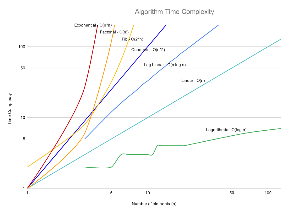
The Algorithm Time Complexity graph below compares several complexity classes over time. A logarithmic scale has been utilized to allow all of the classes to appear in a single image.
Examples of Big O Complexity
O(1) - Constant
O(1) is constant complexity, meaning that the operation is independent of the number of inputs. Operations with constant complexity include
- array access
- array push
- array pop
Functions that perform primitive operations like multiplication, addition, or subtraction also have constant complexity. Below is an example of such a constant function
def isEvenOrOdd(n):
    return "even" if n % 2 == 0 else "odd"
O(log n) - Logarithmic - Dived and Conquer
Algorithms with logarithmic complexity narrow down the search by repeatedly halving n until it there is nothing left to halve. The classic logarithmically complex algorithm is binary search.
def binary_search(self, nums: List[int], target: int) -> int:
    left = 0
    right = len(nums) - 1
    while left <= right:
        pivot = left + (right - left) // 2
        if nums[pivot] == target:
            return pivot
        if target < nums[pivot]:
            right = pivot - 1
        else:
            left = pivot + 1
    return -1
O(n) - Linear Complexity
Linearly complex algorithms scale in proportion to the number of inputs. When there are 100 inputs there are 100 operations. The following functions all have linear complexity.
- Traversing an array
- Traversing a linked list
- Linear Search
In the following example, we’re tasked with finding an integer ‘k’ in an array of increasingly sorted positive integers. Our solution iterates over each value in the array twice which equals 2n. After removing the constant ‘2’ we’re left with linear complexity.
def twoSum(self, nums: List[int], target: int) -> List[int]:
    hashmap = {}
    for i in range(len(nums)):
        hashmap[nums[i]] = i
    for i in range(len(nums)):
        complement = target - nums[i]
        if complement in hashmap and hashmap[complement] != i:
            return [i, hashmap[complement]]
O(n log n) - Log Linear
The best way to understand log-linear complexity is to think of it as linear complexity multiplied by logarithmic. Most of the common sorting algorithms have log-linear complexity.
- merge sort
- heapj sort
- quick sort
Here we have a quick sort implementation that iterates over all values of the array of n length and the values are continually halved.
def quick_sort(arr):
    len_arr = len(arr)

    if len_arr < 2:
        return arr

    current_position = 0

    for i in range(1, len_arr):
        if arr[i] <= arr[0]:
            current_position += 1
            temp = arr[i]
            arr[i] = arr[current_position]
            arr[current_position] = temp

    temp = arr[0]
    arr[0] = arr[current_position]
    arr[current_position] = temp

    left = QuickSort(arr[0:current_position])
    right = QuickSort(arr[current_position + 1:len_arr])

    arr = left + [arr[current_position]] + right

    return arr
O(n2) - Quadratic Complexity
O(n2) is also known at quadratic complexity. This is because performance is proportional to the squared size of the input data. Another way of thinking about it is that it’s linear squared, hence quadratic. This level of complexity often occurs when the data is iterated over in nested loops. There are also several sorting algorithms that have quadratic complexity.
- bubble sort
- insertion sort
- selection sort
A naive solution to the classic Two Sum coding challenge illustrates quadratic complexity. For each element, we try to find its complement by iteratinv through the rest of the array which takes O(n)O(n) time.
def bubblesort(nums):
    for n in range(len(nums) - 1, 0, -1):
        for i in range(n):
            if nums[i] > nums[i + 1]:
                nums[i], nums[i + 1] = nums[i + 1], nums[i]
O(2n) Doubling - Fibonacci
O(2n) represents a function whose performance doubles for every element in the input. Our example is a function which recursive generates the numbers in the Fibonacci sequence. The function recursively calls itself twice for each input number until the number is less than or equal to one.
def fib(target) -> int:
    if target <= 1:
        return target
    return fib(target - 1) + fib(target - 2)
O(n!) - Factorial
Algorithms with O(n!) complexity usually compare each value of n against every other value in the data set. Some solutions to the Traveling Salesman Problem and Finding Permutations of a String have O(n!) complexity.
An O(n!) complexity algorithm to construct all permutations of a string.
def get_permutations(nums):
    def backtrack(first=0):
        if first == n:
            output.append(nums[:])
        for i in range(first, n):
            nums[first], nums[i] = nums[i], nums[first]
            backtrack(first + 1)
            nums[first], nums[i] = nums[i], nums[first]

    n = len(nums)
    output = []
    backtrack()
    return output
O(2n) - Exponential
Finding the exact solution to the Traveling Salesman Problem using dynamic programming has exponential complexity. That solution is non-trivial and won’t be demonstrated here.
Established Values
Every commonly used data structure and search implementation has a well-known complexity. Those complexities are detailed here.
Common Data Structure Operations
| Data Structure | Access (Avg) | Search (Avg) | Insertion (Avg) | Deletion (Avg) |
|---|---|---|---|---|
| Array | O(1) | O(n) | O(n) | O(n) |
| Stack | O(n) | O(n) | O(1) | O(1) |
| Queue | O(n) | O(n) | O(1) | O(1) |
| Singly-Linked List | O(n) | O(n) | O(1) | O(1) |
| Doubly-Linked List | O(n) | O(n) | O(1) | O(1) |
| Hash Table | 0(1) | O(1) | O(1) | O(1) |
| Binary Search Tree | O(log(n)) | O(log(n)) | O(log(n)) | O(log(n)) |
| B-Tree | O(log(n)) | O(log(n)) | O(log(n)) | O(log(n)) |
| Red-Black Tree | O(log(n)) | O(log(n)) | O(log(n)) | O(log(n)) |
| Splay Tree | 0(log(n)) | O(log(n)) | O(log(n)) | O(log(n)) |
| AVL Tree | O(log(n)) | O(log(n)) | O(log(n)) | O(log(n)) |
| KD Tree | O(log(n)) | O(log(n)) | O(log(n)) | O(log(n)) |
Common Search Implementations
| Algorithm | Best | Average | Worse | Space (Worst) |
|---|---|---|---|---|
| Quicksort | O(n log(n)) | Θ(n log(n)) | O(n^2) | O(log(n)) |
| Mergesort | O(n log(n)) | Θ(n log(n)) | O(n log(n)) | O(n) |
| Timsort | O(n) | Θ(n log(n)) | O(n log(n)) | O(n) |
| Heapsort | O(n log(n)) | Θ(n log(n)) | O(n log(n)) | O(1) |
| Bubble Sort | O(n) | Θ(n^2) | O(n^2) | O(1) |
| Insertion Sort | O(n) | Θ(n^2) | O(n^2) | O(1) |
| Selection Sort | O(n^2) | Θ(n^2) | O(n^2) | O(1) |
| Tree Sort | O(n log(n)) | Θ(n log(n)) | O(n^2) | O(n) |
| Shell Sort | O(n log(n)) | Θ(n(log(n))^2) | O(n(log(n))^2) | O(1) |
| Bucket Sort | O(n+k) | Θ(n+k) | O(n^2) | O(n) |
| Radix Sort | O(nk) | Θ(nk) | O(nk) | O(n+k) |
| Counting Sort | O(n+k) | Θ(n+k) | O(n+k) | O(k) |
| Cubesort | O(n) | Θ(n log(n)) | O(n log(n)) | O(n) |